Boundary value problems for parabolic equations with different boundary conditions

Full Text

Boundary value problems for the heat equation are one of the important sections of the equations of mathematical physics. In addition to the classical versions of problems for a homogeneous rod, cases where the rod is inhomogeneous are also interesting. Solving these problems may be of interest for areas related to multilayer structures. For example, such areas are medicine [1] or manufacturing [2] (manufacturing various multilayer parts for which they experience large temperature differences during operation).

Statement of the problem and construction of an analytical solution

Find the temperature distribution along a finite rod composed of two homogeneous rods touching at the point ???? = ????0, with characteristics ???? and ????, respectively. The lateral surface of the rods is thermally insulated, and the ends of the component rods are maintained at zero temperature. The temperature at the initial time in the component rods is different.

The mathematical model of the problem has the form: find the function ,  which is a solution to the equation

$Lu\equiv \left\{\begin{array}{c}{u}_t-a^2{u}_{xx}=\mathrm{0,} 0<x<l_0, 0<t<T,\\ u_t-b^2{u}_{xx}=\mathrm{0,} l_0<x<l, 0<t<T,\end{array}\right. \left(1\right)$

and satisfies the conditions

$u\left(x\mathrm{,0}\right)\equiv \left\{\begin{array}{c}{\phi }_1\left(x\right), 0<x<l_0,\\ {\phi }_2\left(x\right), l_0<x<l, \end{array}\right. \left(2\right)$                 

$u\left(\mathrm{0,}t\right)=u\left(l,t\right)=\mathrm{0,}0<t<T, \left(3\right)$

$u\left(l_0-\mathrm{0,}t\right)=u\left(l_0+\mathrm{0,}t\right). \left(4\right)$

Using the method of separation of variables and the gluing condition, an analytical solution was obtained in the form of a series:

$u\left(x,t\right)=\frac{\left(l-l_0\right)x{{\displaystyle \sum }}_{n=1}^{\infty }{D}_n\left(x, t\right)-l_0\left(l-x\right){{\displaystyle \sum }}_{n=1}^{\infty }{B}_n\left(x, t\right)}{\left(x-l_0\right)l+l_0\left(l-l_0\right)\left({\displaystyle {\sum }_{n=1}^{\infty }{C}_n\left(x, t\right)-{\sum }_{n=1}^{\infty }{A}_n\left(x, t\right)}\right)}+$

$+\frac{l_0\left(l-l_0\right)\left({\displaystyle {\sum }_{n=1}^{\infty }{B}_n\left(x, t\right){\sum }_{n=1}^{\infty }{C}_n\left(x, t\right)-{\sum }_{n=1}^{\infty }{A}_n\left(x, t\right){\sum }_{n=1}^{\infty }{D}_n\left(x, t\right)}\right)}{\left(x-l_0\right)l+l_0\left(l-l_0\right)\left({\displaystyle {\sum }_{n=1}^{\infty }{C}_n\left(x, t\right)-{\sum }_{n=1}^{\infty }{A}_n\left(x, t\right)}\right)} \left(5\right)$

where

$\underset{n=1}{\overset{\infty }{}}{A}_n\left(x, t\right)=\underset{n=1}{\overset{\infty }{}}\frac{2\cdot {\left(-1\right)}^n}{\pi n}{e}^{-{\left(\frac{a\pi n}{l_0}\right)}^{2}t}\sin \left(\frac{\pi n}{l_0}x\right) \left(6\right)$

  $\underset{n=1}{\overset{\infty }{}}{B}_n\left(x, t\right)=\underset{n=1}{\overset{\infty }{}}{B}_n{e}^{-{\left(\frac{a\pi n}{l_0}\right)}^{2}t}\sin \left(\frac{\pi n}{l_0}x\right)=$                                     

$=\frac{2}{l_0}\underset{n=1}{\overset{\infty }{}}{e}^{-{\left(\frac{a\pi n}{l_0}\right)}^{2}t}\sin \left(\frac{\pi n}{l_0}x\right)\underset{0}{\overset{l_0}{}}{\phi }_1\left(s\right)\sin \left(\frac{\pi n}{l_0}s\right)ds \left(7\right)$

$\underset{n=1}{\overset{\infty }{}}{C}_n\left(x, t\right)=\underset{n=1}{\overset{\infty }{}}\frac{2}{\pi n}{e}^{-{\left(\frac{b\pi n}{l-l_0}\right)}^{2}t}\sin \left(\frac{\pi n\left(x-l_0\right)}{l-l_0}\right) \left(8\right)$

$\underset{n=1}{\overset{\infty }{}}{D}_n\left(x, t\right)=\underset{n=1}{\overset{\infty }{}}{D}_n{e}^{-{\left(\frac{b\pi n}{l-l_0}\right)}^{2}t}\sin \left(\frac{\pi n\left(x-l_0\right)}{l-l_0}\right)=$

$=\frac{2}{l-l_0}\underset{n=1}{\overset{\infty }{}}{e}^{-{\left(\frac{b\pi n}{l-l_0}\right)}^{2}t}\sin \left(\frac{\pi n\left(x-l_0\right)}{l-l_0}\right)\underset{l_0}{\overset{l}{}}{\phi }_2\left(s\right)\sin \left(\frac{\pi ns}{l-l_0}\right)ds \left(9\right)$

 

Estimation of the remainder of the series and the number of terms

Let us estimate series (6) - (9) from above. As a result of the assessment, we obtain the following expressions:

$R_N^A=\frac{l_0^2}{a^2{\pi }^3{N}^{2}t}{e}^{-{\left(\frac{a\pi N}{l_0}\right)}^{2}t}$

$R_N^B=\frac{l_0^3}{a^2{\pi }^3{N}^{2}t}{e}^{-{\left(\frac{a\pi N}{l_0}\right)}^{2}t}$

$R_N^C=\frac{{\left(l-l_0\right)}^2}{b^2{\pi }^3{N}^{2}t}{e}^{-{\left(\frac{b\pi N}{l-l_0}\right)}^{2}t}$

$R_N^D=\frac{2{\left(l-l_0\right)}^2}{b^2{\pi }^3{N}^{2}t}\left(l_0+\frac{l}{\pi }\right)e^{-{\left(\frac{b\pi N}{l-l_0}\right)}^{2}t}$

 

These estimates are needed in order to calculate how many terms must be summed to obtain a more accurate solution. The tables show the calculations for two given accuracy ε, different t and the following parameter values: $a=1;b=\mathrm{0,3};l_0=\mathrm{1,7};l=3.$

From the tables it follows that with this choice of parameters, the series converge quickly and, having summed up about 300 and 400 terms, we already achieve good accuracy ε = 0.001 and ε = 0.00001, respectively.

Charting

For plotting, a program was written in the C # programming language using the .NET Framework 4.5 framework in the Microsoft Visual Studio 2019 development environment. The program is a windowed application with fields for entering parameters , time interval T, and buttons, when clicked, the graphs of the dependence  are drawn for a fixed value of t. The simulation results are presented in the figures 1-3.

It can be seen from the figures that a jump in temperature occurs at the point of discontinuity. In this case, the gluing condition is not violated, since the jump does not occur instantly. It can also be seen that as t approaches the end of a given time interval, the value of the function approaches zero, which indicates the establishment of the process.

Conclusion

So, an analytical solution to problem (1) - (4) was obtained and graphs of its visualization were constructed. Therefore, the tasks were completed, the goal of the work is achieved.

 

Table 1

The number of terms at

	$t=1$	$t=\mathrm{0,1}$	$t=\mathrm{0,01}$	$t=\mathrm{0,001}$	$t=\mathrm{0,0001}$
$R_a$	2	4	12	36	113
$R_b$	2	4	12	38	118
$R_c$	3	10	29	91	287
$R_d$	3	10	30	94	297

 

Table 2

The number of terms at

	$t=1$	$t=\mathrm{0,1}$	$t=\mathrm{0,01}$	$t=\mathrm{0,001}$	$t=\mathrm{0,0001}$
$R_a$	2	5	16	50	156
$R_b$	2	6	16	51	160
$R_c$	4	13	40	126	397
$R_d$	5	13	41	129	405

 

Fig. 1. Graph of u (x) at the beginning of the time interval

 

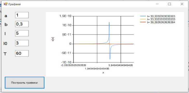
Fig. 2. Graph of u (x) at the middle of the time interval

 

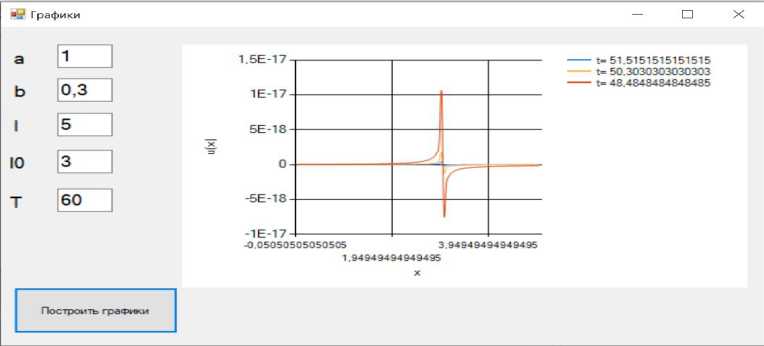
Fig. 3. Graph of u (x) at the ending of the time interval

About the authors

Yuliana Yurievna Krivosheeva

Samara University

Author for correspondence.
Email: akinava.love@gmail.com

graduate student of the Faculty of Informatics

Russian Federation, 443086, Russia, Samara, Moskovskoye Shosse, 34

Natalia Aleksandrovna Slobozhanina

Samara University

Email: slobogeanina@mail.ru

assistant professor of the Department of Technical Cybernetics of the Samara University

Russian Federation, 443086, Russia, Samara, Moskovskoye Shosse, 34

References

Supplementary files